Advances in Optical Techniques for Moisture and Hydrocarbon Detection
|
Andrew M.V. Stokes and Michael D. Summers, Michell Instruments Limited, Ely, UK
 
|
Contents
- Abstract
- Driving Factors for Improved Process Instrumentation for the Natural Gas Industry
- Historic Natural Gas Trends
- Emerging Natural Gas Trends
- Measurement Standards
- What is The “Real” Hydrocarbon Dew Point?
- Phase Envelope of Natural Gas
- The Role of Light and Optics in Moisture and HCDP Measurement
- Interference
- Spectroscopy
- Evanescent Waves
- Conclusion
- References
|
Abstract
|
|
Every year, the world uses in the region of 100 trillion scf (standard cubic feet) of natural gas (1). All of this gas requires treatment before it enters the pipeline, making natural gas processing a key global industry. Minimization of costs is achieved through optimization of these processes, requiring accurate online measurement of gas composition at multiple points in the chain. New proposed guidelines require the development of more sensitive detection limits. The field of optics already plays a large part in existing measurement technologies and further developments promise to provide improved techniques for use in natural gas analysis.
|
Driving Factors for Improved Process Instrumentation for the Natural Gas Industry
|
Raw natural gas varies substantially in composition from source to source. Methane is always the major component, typically comprising 60% to 98% of the total. Additionally, natural gas contains significant amounts of ethane, some propane and butane, and typically 1% to 3% of other heavier hydrocarbons. Often, natural gas contains associated and undesirable impurities, such as water, carbon dioxide, nitrogen, and hydrogen sulfide. Although the composition of raw gas varies widely, the composition of gas delivered to commercial pipeline grids is tightly controlled.
In order for the gas producers to meet pipeline specifications, all natural gas requires some treatment even if all that is done is to remove bulk water. Around a fifth of gas extracted requires extensive, and often expensive, treatment, before it can be delivered to the pipeline. Processing of natural gas is therefore, by some considerable margin, the largest industrial gas application. In the U.S., production of natural gas is presently around 22 trillion scf/yr and expected to increase to more than 31 trillion scf/yr by 2025. It follows that U.S. production accounts for somewhere in the region of 20% of total Global production making the U.S. a key market both for gas producers, processing equipment, and instrumentation suppliers.
|
Historic Natural Gas Trends
|
|
Most natural gas treatment involves the removal of solids, free liquids and the reduction of water vapor content to acceptable levels (typically to 7 lbs water /Mscf. or less), all done before the gas enters the transmission pipeline system. Historically, most natural gas was also processed to separate the heavier hydrocarbon components (ethane, propane, and butanes plus) that could derive higher economic value as natural gas liquids (NGLs) in the petrochemical feedstock market (2). As such, following conditioning, treatment, and processing, natural gas entering interstate commerce was historically a largely fungible commodity (2). Interstate natural gas pipeline tariffs derived from these historical practices, with representative quality standards generally being characterized as shown in table 1, (with certain variances specific to individual pipeline tariffs).
|
Component
(molar %)
|
Minimum
|
Maximum
|
| Methane
|
75
|
-
|
| Ethane
|
-
|
10
|
| Propane
|
-
|
5
|
| Butanes
|
-
|
2
|
| Pentanes plus
|
-
|
0.5
|
| Nitrogen & other inerts
|
-
|
3 - 4
|
| Carbon dioxide
|
-
|
3 - 4
|
| Trace components
|
-
|
0.25 - 1
|
|
Table 1: Typical U.S. tariff limits (3)
|
|
|
For natural gas producers, there is an associated requirement that states that natural gas should be free of liquid water and hydrocarbons at delivery temperature and pressure and free of particulates in amounts deleterious to transmission and utilization equipment.
Within these broad-brush limits, actual gas composition varies significantly from field to field and also dynamically as the methods of extraction can lead to fractional variations, particularly as the field becomes depleted over time. To give an illustration of the range of compositional variations that can be seen, the following examples are provided:
|
|
Gas Component
|
Casinghead (Wet) Gas
(mol %)
|
Gas Well (Dry) Gas
(mol %)
|
Condensate Well Gas
(mol %)
|
|
Carbon Dioxide
|
0.63
|
Trace
|
Trace
|
|
Nitrogen
|
3.73
|
1.25
|
0.53
|
|
Hydrogen Sulfide
|
0.57
|
Trace
|
Trace
|
|
Methane
|
64.48
|
91.01
|
94.87
|
|
Ethane
|
11.98
|
4.88
|
2.89
|
|
Propane
|
8.75
|
1.69
|
0.92
|
|
Iso-Butane
|
0.93
|
0.14
|
0.31
|
|
n-Butane
|
2.91
|
0.52
|
0.22
|
|
iso-Pentane
|
0.54
|
0.09
|
0.09
|
|
n-Pentane
|
0.80
|
0.18
|
0.06
|
|
Hexanes
|
0.37
|
0.13
|
0.05
|
|
Heptanes plus
|
0.31
|
0.11
|
0.06
|
|
Total
|
100.00
|
100.00
|
100.00
|
|
Table 2: Typical raw gas composition (3)
|
|
Emerging Natural Gas Trends
|
However, all shale gas is not the same in terms of its composition, and therefore also varies with regard to its processing requirements. As well as being markedly different from site to site the gas composition often varies significantly across the field (5), for example in the Marcellus shale the gas becomes richer from east to west.
The initial shale gas discovery region was at Barnett shale where gas was first extracted in a core area on the eastern side of the resource play. As drilling has moved westward, the composition of the hydrocarbons in the Barnett shale has varied from dry gas-prone in the east to oil-prone in the west (5).
|
Well
|
C1
|
C2
|
C3
|
CO2
|
N2
|
|
1
|
80.3
|
8.1
|
2.3
|
1.4
|
7.9
|
|
2
|
81.2
|
11.8
|
5.2
|
0.3
|
1.5
|
|
3
|
91.8
|
4.4
|
0.4
|
2.3
|
1.1
|
|
4
|
93.7
|
2.6
|
0.0
|
2.7
|
1.0
|
|
Table 4: Barnett Shale Gas Composition (5)
|
|

Figure 3: Shale basins in the lower 48 states (4) |
|
Table 4 shows the composition of four wells in the Barnett. These wells appear from east to west with the eastern most well on the top (Well No. 1). As the table suggests, there is a large increase in the percentage of ethane and propane present in the westernmost wells. One well sample on the western edge of the resource play (Well No. 4) also shows a high level of nitrogen, approaching 8%. This level is high enough to require treating, but blending with other gas in the area is the most economical solution (5).
|
|
Well
|
C1
|
C2
|
C3
|
CO2
|
N2
|
|
1
|
27.5
|
3.5
|
1.0
|
3.0
|
65.0
|
|
2
|
57.3
|
4.9
|
1.9
|
0
|
35.9
|
|
3
|
77.5
|
4.0
|
0.9
|
3.3
|
14.3
|
|
4
|
85.6
|
4.3
|
0.4
|
9.0
|
0.7
|
|
Table 5: Antrim Shale Gas Composition (5)
|
|
In some fields, like the Antrim shale, gas is predominately biogenic: methane is created as a bi-product of bacterial consumption of organic material in the shale. Significant associated water is produced, requiring central production facilities for dehydration, compression, and disposal. Carbon Dioxide is a naturally occurring by-product of shale gas produced by desorption. It is expected that the CO2 levels in produced gas will themselves increase steadily over the productive life of a well, eventually exceeding 30% in some areas (5).
It follows that as shale gas can vary significantly from area to area; the gas processing requirements for it will also be different from site to site and perhaps even across a single site. Therefore, the demands placed on measurement equipment will also vary significantly across the industry in the future as shale gas becomes an ever increasing part of the market.
|
Measurement Standards
|
There is pressure within the natural gas industry as a whole to establish better measurement standards and practices. Examples of these initiatives, and a brief summary of their scope of work, and likely outcome(s), are as follows:
GERG Project 1.70: Expansion of the experimentally validated application of the GERG Water equation of state to cover the dew point range from -50 to +80°C and 1 to 250 bar (moving on from current -15 to +5°C and 0 to 100 bar). This is expected to result in revision of ISO 18453 with a likely timescale for publication during 2014.
CEN/TC 234 WG 11 Gas Quality: Reviewing the current gas quality parameter specifications stipulated by the EASEE-gas Common Business Practice – 2005-001/01 – Harmonisation of Natural Gas Quality, and will be applicable to transmission gas transfer into and across all EU states. The outcome of this work is expected to result in a change from the present water dew point limit of -8°C at 70 barg (-45°F at 1015 psig) to moisture content 50mg/m3 for pressure conditions greater than 10 barg (160 psig), 200 mg/m3 for lower pressure distribution networks.
EURAMET ENG01 Gas – Characterisation of Energy Gases – Work Package 3: New Primary and reference humidity facilities: Development of humidity calibration facilities for water dew point within natural gas and other energy gases and at pressure to enable dew point sensors and process moisture analysers to be calibrated under simulated process measurement conditions, rather than air at atmospheric pressure.
GERG Project 1.64: Installation, calibration and validation guidelines for on-line hydrocarbon dew point analysers – Phase 1 completed, Phase 2 underway. Harmonization of automatic on-line HC dew point measurement to a specified sensitivity of 5mg/m3 potential hydrocarbon liquid content (PHLC).
These initiatives are likely to have a large impact on the measurement requirements of hydrocarbon dew point and water content of natural gas. It is likely that both measurements will need to be performed with higher sensitivity than is currently typically achieved. However, we will first briefly summarise the present state of the art.
|
What is The “Real” Hydrocarbon Dew Point?
|
The current definition of hydrocarbon dew point agreed by the International Organization for Standardization (ISO) Standard is the: “Temperature above which no condensation of hydrocarbons occurs at a specified pressure” (7)*. This definition can be considered to be equivalent to the temperature at which the first molecule of liquid condensate forms – however it is clear that for all practical purposes, such an occurrence would be extremely difficult to detect experimentally.
Having said that, it is not possible to calibrate commercially available hydrocarbon dew point analysers in a directly traceable way, because no hydrocarbon dew point reference material or a reference instrument is available. Because of differences in working principles, analysers from different manufacturers may give different values for the hydrocarbon dew point for a given gas. In practice, the dew point of an automatic dew point monitor is often “tuned” to match the value measured by a manual chilled mirror, or “tuned” to the value calculated from a known gas composition using a thermodynamic model (8).
*This definition is appended by two Notes:
(1) At a given dew point temperature there is a pressure range within which retrograde condensation can occur. The cricondentherm defines the maximum temperature at which this condensation can occur.
(2) The dew point line is the locus of points for pressure and temperature which separates the single phase gas from the biphasic gas-liquid region.
The techniques used in the field determination of HCDP are either based on direct measurement, or indirect measurement. There are two main methods of direct measurement: instruments based on cooled-mirror techniques and those based around spectroscopy. Existing cooled-mirror based instruments available on the market, be they manual or automatic, measure hydrocarbon dew point (HCDP) directly according to the ISO definition. However, they require more than a single molecule of condensate to be detected, and therefore will typically return a value that is lower than the ‘true’ value. Although all chilled mirror instruments detect the onset of the condensation process directly, by definition they depend on the availability of sufficient material in the vapour phase to form a detectable film. This is quantified by the ‘condensation rate’ of the mixture, which is a measure of the density of condensate formed per °F of temperature change below the HCDP. The variation may be small, typically 1.8-5.4°F, and is generally well within the required industry uncertainty limits, but it can become significant when put in the context of reducing overall gas processing costs. It will also become increasingly significant as the emerging new industry guidelines come into force, particularly GERG 1.64, which will be discussed further in due course. Spectroscopic techniques for HCDP measurement are emerging and are expected to become more established in time. They will also require a finite level of condensate to operate, but should offer more sensitivity fundamentally. In both cases it is necessary to consider how well each technology deals with gas compensation variation and also to bear in mind any additional consumables or servicing that may be necessary as these can add significantly to the overall total cost of ownership per installed measurement point.
Alternatively, indirect methods of HCDP measurement can be deployed. The basis of all indirect methods is the use of a gas chromatograph (GC) to determine the composition of the mixture, and then the use of a thermodynamic equation of state to calculate the condensation curve. Although the composition of the gas can be determined with very high accuracy, (11)(12)(13)(14) it is well known that the overall accuracy of the result depends largely on the validity of the equation of state used, and that different EOS will derive a different predicted value. Additionally, since the hydrocarbon dew point is highly sensitive to the presence of heavier (C6+) hydrocarbon components, which may be present at levels that are below the limit of detection of the GC, there is a significant risk that these methods might be biased. This is particularly true for the so-called C6+ Field GC, most commonly used in on-line measurements.
|
Phase Envelope of Natural Gas
|
The temperature and pressure at which the HCDP occurs follows a curve that forms a so-called phase envelope, the exact form of which is unique to any given gas composition. Within the phase envelope, condensate will be formed at any point to the left of the dew point curve. The further left in the phase envelope the operating conditions are, it follows that more condensate will form.
It is usual to refer to the maximum temperature for any pressure at which condensate is formed as the cricondentherm, which also varies with composition.
However, as the red line constitutes the temperature at which the first molecule of liquid would condense, it is more useful to consider a family of curves such as those shown on the right.
|
Figure 6: Typical phase envelope** |
These represent the relationship between the concentration of total potential condensate in a given volume of gas (here shown in mg/m3) and the corresponding temperature. Existing automatic HCDP Analyzers have been proven to work reliably and repeatably in the 20 to 70 mg/m3 range (9)(10).
From the chart, it is clear that the difference between the 20 mg/m3 line and the 5 mg/m3 line at the typical measurement pressure of 392 psig (27 barg), which is the most common analysis pressure utilised across the industry, equates to between -3.2°F (-27°C) and -8°F (-5°C).
|

Figure 7: Phase envelope showing relationship to condensation rate 8 |
** The dew point line is the locus of points for pressure and temperature which separates the single phase gas from the biphasic gas-liquid region.
As gas producers continually strive to comply with tighter production tolerances, and to comply with the likely recommendations of GERG 1.64, it will be necessary to detect HCDP at, or lower than, the condensation rate of 5mg/m3. These will require increases in sensitivity compared to what can presently be achieved by automatic chilled-mirror technology.
|
Measurement of Moisture Content
|
|
Compared to the measurement of HCDP, the measurement of moisture has inherently far greater traceability with test houses and manufacturer’s having traceable links back to National standards. The main point of note when considering the current, and emerging, needs of the natural gas industry however is that all moisture calibrations are presently performed at atmospheric pressure. Secondly, the majority of analyzers are calibrated in inert gas (typically N2 or air). This can lead to significant errors and is the reason for the work of EURAMET ENG01. |
Figure 8: Relationship between moisture contentand T for air and natural gas |
There are a diverse range of technologies for the measurement of moisture in natural gas, including impedance and capacitive sensors, chilled mirror, quartz crystal micro-balance, and tuneable diode laser spectroscopy. Each measurement technique has its advantages and disadvantages, most of which are widely known. |
Impedance sensors are generally low-cost and very robust, particularly when operating at line pressure with a typical impedance transmitter being able to work at pressures up to 4,500 psig or higher without degradation in performance. An important consideration for natural gas processing is that these transmitters are available in hazardous area approved configurations. Accuracy is typically 1.6 to 3.2°F and devices usually have a wide measurement range, commonly -148/+68°F. Other drawbacks associated with this technology include: poor long term measurement stability; the need for periodic sensor recalibration; and susceptibility to contamination, making appropriate sample conditioning critical.
Cooled-mirror hygrometers are fundamental by nature, so offer good accuracy, however they are limited in range by the thermoelectric cooling modules typically used to control the mirror surface temperature onto which the condensate is sublimated. They can also take a moderate to long time to reach steady state equilibrium, this response time being directly related to the amount of moisture present in the gas being measured: the lower the moisture level the longer the response. Cooled-mirror analyzers typically need to be installed in a purged enclosure for use in hazardous areas so they are not ideally suited for use in the natural gas industry.
Quartz crystal micro-balance (QCM) analyzers are pseudo-fundamental, relying as they do on a mass determination. However they measure dynamically by comparing frequency shift periodically from a dry reference to the process gas so cannot truly be considered as an absolute measurement. They are fast to respond, particularly to increasing moisture levels but can take a long time to dry down due to system response dynamics. Typically accuracy from a QCM analyzer is ±10% of reading from 1-2,500 ppmV (parts per million by volume). QCM analyzers require very precise flow and pressure control to work accurately and also suffer from a low working pressure range typically being limited 30 psig maximum (2 barg). They also require periodic replacement of desiccant material and/or the moisture permeation device used for auto-compensation, all of which adds significant complication to any measurement point.
Tunable diode laser absorption spectrometers (TDLAS) offer several advantages, and can be considered to be a fully non-contact method of continuous moisture measurement in natural gas. The principle is inherently fundamental, being based on a direct measurement of fractional absorption by each gas component. TDLAS analyzers also offer a fast response time with typical measurement periods on the order of seconds. However, real-world response tends to be governed mainly by system response characteristics, such as gas flow rates, so often response times would be slower than theory suggests. Although, due to their molecular selectivity, they can be considered immune to contamination effects, TDLAS analyzers can suffer from significant interference in complex mixtures such as natural gas, due to the spectra of other species present in the gas composition. Although care is taken to select the most appropriate wavelength to maximise absorption by the species of interest while minimising any interference from other components in the gas mixture, interference usually sets a lower bound on detection limits and accuracy in natural gas applications.
For trace moisture measurement in natural gas, the most significant factor is CH4 which has a peak very close to the one often used for moisture determination. The effect of this is that TDLAS analyzers often need to be calibrated specifically for the gas composition on which they will be used. As has been mentioned in this paper, natural gas composition can vary dramatically, either due to variation in field dynamics or due to blending / mixing during processing or transportation. Any deviation from the gas composition that was used for calibration will result in measurement errors. These could become considerable over the range of compositions that have been presented and will no-doubt be more noticeable for shale derived gas. Accuracy of the current generation of field TDLAS analyzers is generally good but can deteriorate as the limit of sensitivity is reached, for example a typical low moisture detection limit for a TDLAS may be 5ppm with a claimed accuracy of +/-4ppm. This represents an overall uncertainty of measurement corresponding to 1 to 9ppm, which in dew point temperature terms equates to -105 to -78°F (-76.2 to -61.3°C).
A final point to mention is that most TDLAS analyzers work at atmospheric pressure only, which can be a problem if gas needs to be vented into a flare stack or some form of re-integration downstream of the measurement. Some work at reduced pressure in the region of 100mbar necessitates the uses of a vacuum pump in the gas handling system: an expensive component and one that is potentially unreliable and/or requires high levels of maintenance during the lifetime of the installation.
Maintenance is a big consideration when evaluating the lifetime costs of the different measurement technologies, both for moisture and HCDP measurement. As more customers outsource the maintenance function within their plants, they continually look to install low
maintenance equipment. It is clear that, although the initial purchase cost of a particular analyzer is a primary concern, thought should also be given to the true total cost of ownership of the instrument over its likely lifetime. Aspects that should be taken into account include: Installation costs; Service costs; Periodic recalibration costs; Consumables including calibration and/or reference gases; Sample conditioning costs.
The natural gas industry is moving forwards and its needs are evolving as the market develops. Measurement technologies need to adapt and improve in step with the industry. To this end, Michell Instruments are targeting their research at developing a new generation of moisture and HDCP sensors incorporating the strengths of multiple existing techniques, along with more recent advances in optical technology.
|
The Role of Light and Optics in Moisture and HCDP Measurement
|
From an optics perspective, there are two different condensate systems to deal with. The first is moisture condensate, which takes the form of droplets due to the large surface tension of water. In moisture dewpoint chilled mirror sensors, water condenses onto a mirror surface and the resulting spheroidal droplets tend to scatter light strongly, generating a change in the detected signal. In the event of crystal formation (ice or gas hydrates), there is a similar degree of scattering, making it difficult to differentiate. The second type of measurement performed using chilled surface sensors is on hydrocarbon (HC) condensate which forms thin films of low viscosity. These are difficult to detect optically so simple scattering measurements aren’t as practical and other strategies are used.
One approach is to form HC condensate films on a roughened surface. If a surface is perfectly “matte”, then reflected light is scattered randomly, leading to a Lambertian (diffuse) distribution of reflected light. A reflective surface will produce a specular (mirror-like) reflection, with the reflected light leaving the surface at the same angle as the incident light, relative to the reflector. As the film forms on the roughened surface, it fills in the dips in the rough surface until a distinct layer has formed. The interface between the liquid layer and the gas provides a surface layer capable of providing a specular reflection. Schemes have been devised to increase the contrast between the two cases (diffuse and specular), such as adding conical depressions in the surface to produce dark regions in the reflected optical field in the presence of condensate15.
For both types of chilled surface measurement, the optical surface is thermally bonded to a thermoelectric cooler (TEC), usually a Peltier device. This pulls heat from the top surface (and whatever is bonded to it) and transfers it to the opposite side, which is usually bonded to a heat sink. The amount of heat transferred is controlled by a voltage level sent to the TEC. Feedback from a temperature sensor is used to create a control loop which stabilises the cooler at a set temperature, or to scan through a set rate of change in temperature. To stabilise the cooling characteristic, a Proportional-Integral-Derivative (PID) control loop is the usual approach.
As far as measurement is concerned, the aim is to generate an optical response signal using as little condensate as possible. Clearly, the volume of condensate required to make a measurement in this manner varies with the depth of the surface features which need to be filled before a reflective surface can be formed. It is therefore desirable to optimise the chilled surface to be exactly just rough enough to create a Lambertian profile for the illuminating light. To provide immunity to local variations in the surface, perhaps caused by residue or other contamination being left on the surface, it is also useful to use a fairly large surface area. Of course, the downside is that a larger surface area requires more energy to cool and can introduce additional uncertainty in the precise surface temperature.
The limiting factor for many optical measurement techniques, including those used in many existing chilled mirror systems is the wavelength of the light used. Electromagnetic waves don’t interact with objects that are much smaller than their wavelength. Visible light is in the range of 400-700nm (approximately 0.02 thousandths of an inch) and won’t scatter or diffract due to objects smaller than that. It is therefore advantageous, when practical, to use shorter wavelengths when making most optical measurements. However, there are several features of light which we can exploit to get around this “diffraction limit”.
|
Interference
|
When discussing light, as with all electromagnetic radiation, one of the descriptions we use is the wavelength. The wave-like nature of light gives rise to a number of interesting phenomena. Perhaps the most significant of these is interference. When multiple waves interact, they result in a wave that is a combination of all the waves superimposed (see figure 9, below). Coherence is another property of light important to interference effects and is a measure of the continuity of the wave train emitted by the light source. Regular glitches in the wave introduce sudden relative phase shifts between interfering beams, ruining any interference pattern. Lasers tend to produce light with a long coherence length (the average distance between glitches) and therefore tend to be used in interferometric applications.
Figure 9: The wave nature of light. Left: When two waves interact, they produce a wave with amplitude equal to their sum. When they are exactly in phase, they reinforce and when out of phase, they cancel each other out. Right: Interference is reliant on coherence, which is a measure of the continuity of the waves. Certain light sources, such as lasers, produce highly coherent light, which is required for many interferometric measurements.
If we imagine a situation where one of the waves in phase-shifted a small amount relative to the other, we could generate a relatively large change in signal for a phase shift of only a fraction of a wavelength. We only require a means of creating this phase shift.
In 1887, Albert Abraham Michelson developed an optical arrangement which is now named after him. In a Michelson Interferometer16 (see figure 10, below), light from a single source is separated into two separate paths using a beam-splitter, reflected back on themselves, recombined at the beamsplitter and then viewed (by eye, or a suitable sensor). When the recombined light is projected onto a surface (such as a camera), a series of light and dark fringes can be observed. This can be thought of as a “contour plot” showing the difference in path for the two interfering light paths. For instance, if one mirror is tilted with respect to the other, a pattern of stripes is generated, with the distance between each dark fringe corresponding to a difference in height of half a wavelength. Similarly, as the separation of the two mirrors changes through constructive and destructive interference conditions, the projected fringes will switch between light and dark.
If instead of physically moving a mirror, you condense a liquid on its surface, you can create the same effect by virtue of the fact that the refractive index of the liquid is greater than that of the air it displaced. This is because light travels more slowly through materials of a higher refractive index, resulting in a longer effective path length, which depends on the quantity of condensate present.


Figure 10: An illustration of a Michelson interferometer. (Top left) The measurement mirror, M1, is tilted with respect to the reference mirror, M2. This results in a series of vertical fringes in the imaging plane. (Top right) A droplet forms on the measurement mirror, creating a circular interference pattern.(Bottom) Example of a video capture showing the signal change due to the evaporation of a hydrocarbon film deposited on the measurement mirror of an interferometer.
|
Spectroscopy
|
A basic spectroscopic system consists of a light source, a measurement cell, and a light detector. By selecting the wavelength of the light source to match the absorption spectrum of the substance you are trying to detect, you would expect the signal on the detector to decrease if your target substance is present. In terms of a chilled surface sensor based around a light source and detector, there may be some merit in selecting a wavelength of light which is absorbed by the condensate, thus generating a larger change in signal than would be obtained from scattering alone. This becomes especially attractive if you need to distinguish between multiple different substances that may be present, such as water and hydrocarbons.


Figure 11: (Top) An illustration of light absorption through a gas cell. (Bottom) A graph of
light transmission as a function of wavelength through a 1m long cell containing 1000 ppm
of methane.
As the change in signal is dependent on the quantity of substance between the source and
the detector, there is a distinct advantage to be gained by increasing the path (interaction
length) the light has to take through the measurement cell. The relationship between the
signal leaving the source and the signal reaching the detector (I) is described by the Beer-
Lambert Law.
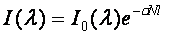 [1] [1]
Where I0 is the light intensity at the source (as a function of wavelength), λ), σ is the
absorption cross-section of the substance at that wavelength (a measure of how strongly it
absorbs light), N is the linear density of the absorbing particles and l is the optical path
length through the sample. In other words, the fractional change in signal due to
spectroscopic absorption at a given wavelength (T) is dependent on the distance through
the sample that the light has to travel.
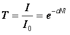 [2] [2]
Once an appropriate wavelength is selected, the best way to achieve this increase in signal
without making the sample cell unwieldy is to add mirrors to reflect the light backwards and
forwards through the sample. However, care must be taken to avoid or handle interference
effects which occur if the beam path overlaps. Enhanced path lengths of 10 to over 100
passes can be achieved using a multi-pass optical cell, often referred to as a Herriott cell
(see Figure 11, below). These use mirrors at each end of the sample and are designed to
avoid overlap between the various beam reflections. For path lengths consisting of 1000’s of
passes, optical cavity arrangements are used. These ensure that the reflected waves overlap
each other, but control the relative phase of the reflections so that they interfere
constructively, or in a predictable manner. To achieve a very long effective path length,
these require specially designed highly reflective mirrors (more than 99.99%, compared to
98% for a typical metallic mirror).
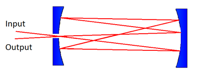
Figure 12: A basic diagram illustrating a multi-pass Herriott-type cell
Although these sorts of path-length enhancement techniques have been developed for use
in gas spectroscopy, they can be readily adapted for optical surface sensors. The other
advantage of making these measurements with liquid condensate is that the density of
molecules is higher than for a gas, so signal change is proportionally greater.
|
Evanescent Waves
|
Another phenomenon peculiar to electromagnetic radiation which can be exploited for chilled
surface measurements is the evanescent wave. This effect is a consequence of total internal
reflection which occurs when light (or electromagnetic radiation) propagating through a
material of a high refractive index (nhigh), such as glass (n=1.5) reaches an interface with a
lower refractive index (nlow), such as air (n=1.001) at an angle greater than a critical angle,
Θc, where
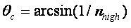 [3] [3]
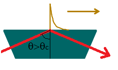
Figure 13: An illustration of total internal reflection generating an evanescent wave which
propagates in the same direction along the interface
This total internal reflection is most commonly used in optical fibres, where it used to
channel light down a high refractive index glass core, surrounded by glass of a lower
refractive index, with very little loss. Although this is a very effective way of reflecting light,
it is not a complete description of what happens at the interface.
Instead of folding neatly at the surface, the wave nature of the light means that the
electromagnetic field penetrates the low refractive index medium as it “bends” around the
interface, for a distance approaching a wavelength. This penetrating wave intensity decays
exponentially away from the surface and is known as an evanescent (or “vanishing”) wave.
This evanescent field is sensitive to changes on the interface, such as the formation of
condensate in much the same way as normally propagating light. These losses can be due
to scattering or spectroscopic absorption. In addition, any losses in intensity of the
evanescent wave translate to losses in the propagating light. This means that absorption
taking place in the evanescent field can be measured in the same way as other sensors,
using a simple photodiode. In addition, the evanescent field can interact with objects and
layers much smaller than the wavelength of the light used, beating the diffraction limit
associated with other light-scattering phenomena.
The following arrangement was recently used to characterise evanescent light scattering on surfaces by van Leeuwen et al17, can be readily adapted to perform this sort of absorption or scattering loss measurement (see figure 14, below). In addition, this arrangement utilises a cavity feedback arrangement which increases the effective path length by a factor of 100. The reflected waves are kept in phase by placing one of the mirrors on a piezoelectric transducer (PZT), which rapidly adapts the length of the cavity to maintain a maximum signal on the photodiode, which only occurs when the resonating waves interfere constructively.
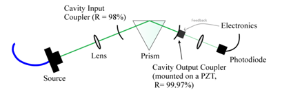 

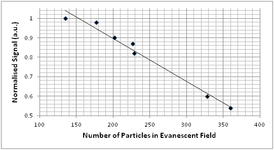
Figure 14: (Top left) An optical arrangement for generating a cavity-enhanced evanescent wave at the surface of a prism. (Top right) An image of light scattered from the evanescent field, taken from above. (Center) Images taken from above the prism using a microscope showing the accumulation of scattering particles with time. (Bottom) Plot of relative photodiode signal with number of particles in the evanescent field. Experimental details presented with permission from the Ritchie Group at the Department of Chemistry at the University of Oxford.
In this experiment, microscopic particles of silica (radius of 500 nm) were used to scatter light out of the evanescent field resonating between the two mirrors. These particles were drawn into the evanescent field due to the optical gradient in a phenomenon known as optical trapping. As the number of particles in the evanescent field increased, the light reaching the photodiode decreased in a linear fashion.
|
Conclusion
|
|
With the position of natural gas as a key source of energy globally, there is a great need for effective analysis of gas composition and the associated cost of gas processing. Due to the sheer scale of the industry, optimizing these processes can result in correspondingly large gains in cost efficiency. As new guidelines governing gas measurement standards and practices come into effect, there will be an increased demand for reliable, robust, and accurate sensors for the gas industry. We have outlined many of the approaches that could be used to enhance and replace existing technologies, purely through the application of more sophisticated optical techniques.
|
References
|
- “Natural Gas Processing with Membranes: An Overview”, Richard W. Baker and Kaaeid Lokhandwala
- “Interstate Natural Gas — Quality Specifications & Interchangeability”, Center for Energy Economics, December 2004
- “The Gas Processing Industry: Its Function and Role in Energy Supplies”, Gas Processors Association
- “Natural Gas Plays in the Marcellus Shale: Challenges and Potential Opportunities”, David M. Kargbo, Ron G. Wilhelm, David J. Campbell
- Composition Variety Complicates Processing Plans for US Shale Gas, Keith Bullin PhD, Peter Krouskop PhD, Bryan Research and Engineering Inc.
- Adapted from Ronald J. Hill, Daniel M. Jarvie, John Zumberge, Mitchell Henry, and Richard M. Pollastro Oil and gas geochemistry and petroleum systems of the Fort Worth Basin, AAPG Bulletin, v. 91, no. 4 April 2007, pp. 445–473.
- International Standard ISO 14532:2001, Natural gas – Vocabulary
- ISO/TR 12148/2009 “Natural Gas – Calibration of chilled-mirror type instruments for hydrocarbon dew point (liquid formation).”
- “Measurement of the hydrocarbon dew point of real and synthetic natural gas mixtures by direct and indirect methods”, Andrew S. Brown, Martin J. T. Milton, Gergely M. Vargha, Richard Mounce, Chris J. Cowper, Andrew M. V. Stokes, Andy Benton, Dave F. Lander, Andy Ridge and Andrew Laughton
- “Measurement of the hydrocarbon dew point of real and synthetic natural gas mixtures by direct and indirect methods”, Andrew S. Brown, Martin J. T. Milton, Gergely M. Vargha, Richard Mounce, Chris J. Cowper, Andrew M. V. Stokes, Andy Benton, Dave F. Lander, Andy Ridge and Andrew Laughton.
- “Measurement Results of the Michell Condumax II Hydrocarbon Dew Point Analyser and Development of a Direct Relationship between HDP and Potential Hydrocarbon Liquid Content”, Henk-Jan Panneman, Ph.D., N.V. Nederlandse Gasunie
- ISO23874 2006 - Natural Gas – Gas Chromatographic requirements for HC dew point calculation
- A.S. Brown, M. J. T. Milton, C. J. Cowper, G. D. Squire, W. Bremser and R. W. Branch, J. Chromatogr. A., 2004 (1040) 215-225
- G. Vargha, M. J. T. Milton, M. Cox and, S. Kamvissis, J. Chromatogr. A., 2005 (1040) 239-245
- M. J. T. Milton, P. M. Harris, A. S. Brown and C. J. Cowper, Meas. Sci. Tech., submitted for publication, 2008
- Banell et al, “Apparatus for measuring dew-point of a gas stream through light scattering,” United States Patent 4799235. (1986)
- Michelson, A. A., and Morley, E. W., “Relative motion of Earth and luminiferous ether”,Am. J. Science 34, 333, (1887)
- Van Leeuwen, N.J. et al, “Near-field optical trapping with an actively-locked cavity,” Journal of Optics 13 044007 (2011)
Copyright: Michell Instruments Limited, Ely, UK - 2013
Back to top
|
|
|